Lattice Boltzmann Method (LBM)
Flow Analysis in nTop leverages the Lattice Boltzmann Method (LBM) for complex geometry handling, reduced mesh dependency, and efficient parallel computing.
Let’s dig into LBM before running our own flow analyses in nTop.
Analysis at the Mesoscopic Scale
We can approach fluid dynamics at three distinct scales: microscopic, mesoscopic, and macroscopic.
-
Microscopic
-
Mesoscopic
-
Macroscopic
Approaching fluid dynamics at the microscopic view uses molecular dynamics, tracking the movement and interactions of individual atoms or molecules, governed by Newton’s laws of motion.
This approach is computationally intensive, limiting its application to very small spatial and temporal scales or specialized applications where molecular-level interactions are crucial.
The Lattice Boltzmann Method (LBM) offers a powerful alternative by operating at the mesoscopic level. It bridges the gap between molecular dynamics and conventional fluid mechanics, simulating fluid flow through discrete particle distributions.
Traditionally, engineers have modeled fluid dynamics through macroscopic equations, such as using the Finite Volume Method (FVM) to solve the Navier-Stokes equation.
These approaches describe fluid as a continuous medium, dealing with observable properties like velocity, pressure, density, and viscosity that represent the average behavior of large numbers of particles.
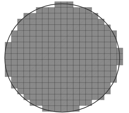
Discretization for LBM
Rather than relying on complex and computationally expensive meshing algorithms, LBM models efficiently subdivide a fluid domain into a Cartesian grid composed of equally sized cells. Each cell represents a discrete location where the particle distribution functions are tracked.
The particle distribution functions are based on the Lattice-Boltzmann Equation (LBE):

c: discrete velocity
x: position
t: time
Ω: collision operator
Each cell within this grid has distribution functions arranged in specific velocity sets. Each direction stores a particle distribution function that represents the probability of finding particles moving in that direction.
You’ll often see LBM models denoted as “DnQm” where:
- m = number of discrete velocities
- n = number of dimensions (2D or 3D)
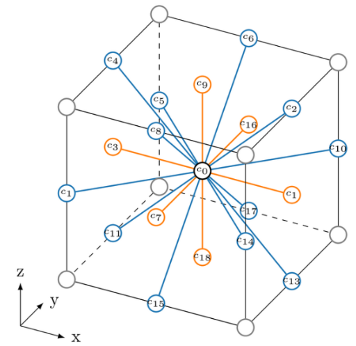
D3Q19 is a common 3D model with 19 discrete velocities, including a zero velocity.
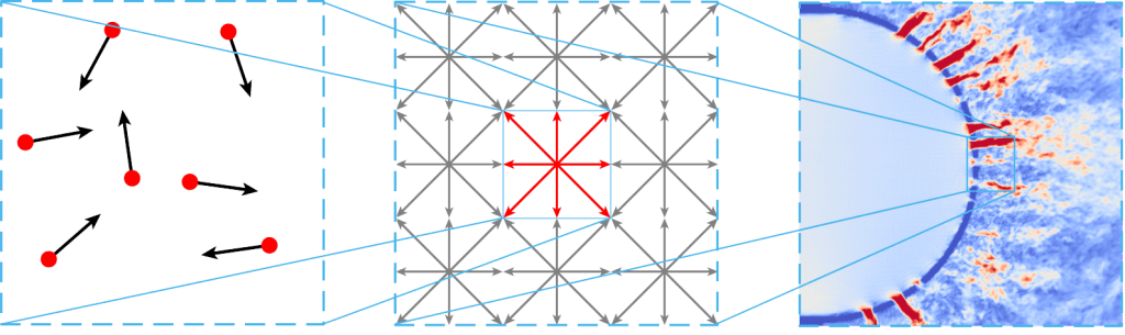
Collision and Streaming
There are two major steps in the LBM algorithm, collision and streaming, that represent fluid particle behavior at each of these discrete locations.
Collision captures how particles in each cell redistribute their momentum through microscopic interactions while conserving mass and momentum.
Streaming connects neighboring cells and represents the fluid particle advection (density, momentum) through the domain.
These alternating processes create the characteristic space-time evolution of the fluid dynamics.
This approach offers several advantages:
✅ Simplified Algorithms: The regular structure allows for more straightforward implementation of the collision and streaming steps.
✅ Complex Geometries: Representing complex boundaries simply requires defining a consistent cell size to capture volumetric features.
✅ Computational Efficiency: The regular structure is particularly well-suited for GPU implementation and parallel computing.
GPU Implementation & Parallel Computing
nTop’s implementation of LBM on GPUs unlocks dramatically faster simulation times; often 10-100x faster than CPU implementations. The chart to the right shows performance on two NVIDIA GPUs. 1000 Million Lattice Updates per second (MLUPs) means that you can compute 1000 Iterations on 1 million cells in one second.

This allows users to handle larger, more complex simulation domains without prohibitive runtime, and to achieve real-time or near-real-time results for certain problem sizes, enabling interactive exploration.