Parametric Blisk Analysis
In this lesson, we will walk through an example of how to set up a thermal and structural analysis of the parametric blisk that was created earlier. The mounting holes in the Parametric Blisk file has been modified slightly to make them cyclically symmetric and export bodies for easier analysis setup.
Downloadable File:
This file was last updated in nTop 5.42.2
1. Generate the Parametric Blisk
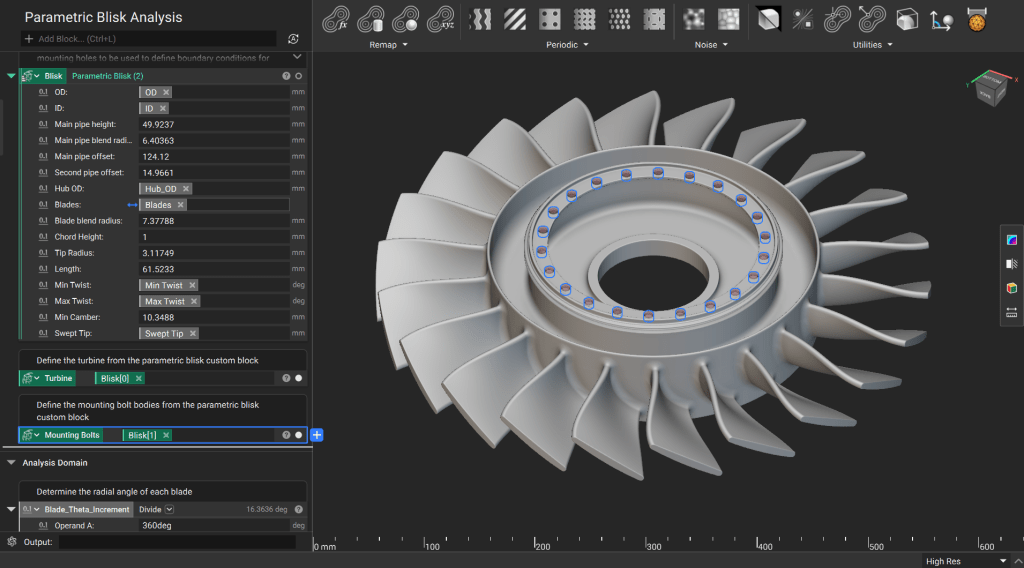
Generate the parametric blisk using the updated custom block. This custom block now outputs a list of implicit bodies – the first element is the blisk, the second element is a polar array of cylindrical bodies at the mounting holes.
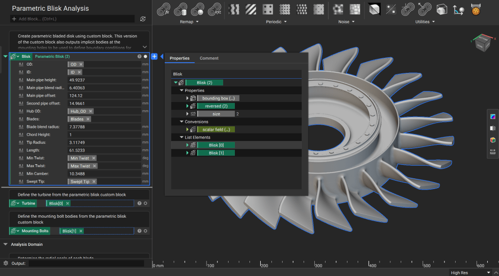
From the properties tab of the Parametric Blisk custom block, drag the first list element into a variable named “Turbine” and the second list element into a variable named “Mounting Bolts”
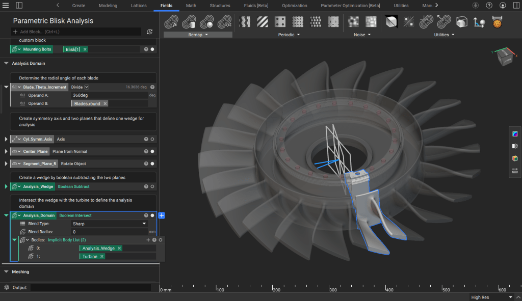
2. Create a Wedge for Analysis
Calculate the angle for each cyclically symmetric wedge for analysis, then rotate a plane from the center coordinate system and perform boolean operations to get just a single wedge.
3. Generate a FE Mesh
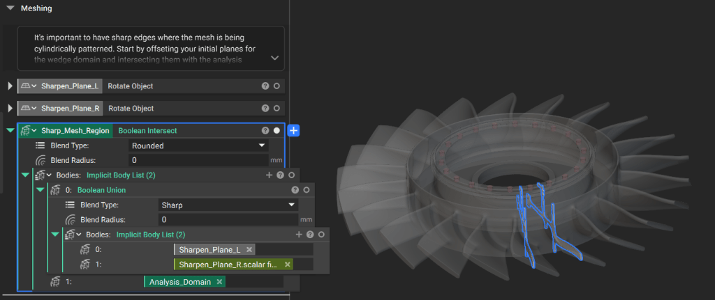
Start by creating an implicit body that can be used to define the “Sharp Extents” of the mesh from implicit body. Do this by rotating the original slice planes slightly and doing a boolean intersect with the analysis wedge.
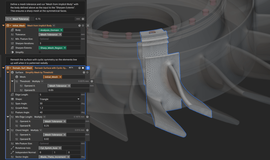
Use the “Mesh from Implicit Body” block to create an initial mesh, using the body created above as the input for “Sharpen Extents”. Then use the “Remesh Surface with Cyclic Symmetry” block to ensure the triangles in the mesh are cyclically symmetric.
Turn the surface mesh into a volume mesh and then into a FE Volume mesh to be analyzed
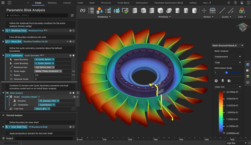
4. Define Boundary Conditions for Structural Analysis
Specify material to create an FE Solid Domain and then define you cyclically symmetric faces on either side of the wedge and your displacement restraint on the bolt holes.
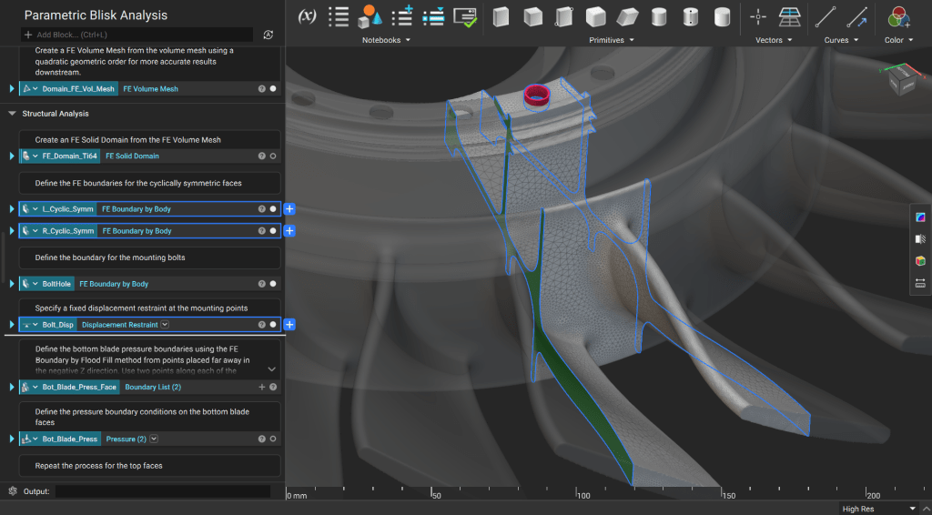
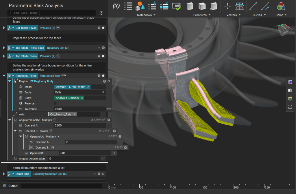
Next define the pressure boundary conditions on either side of the blade faces and a rotational force boundary condition on the entire wedge.
Finally define your Cyclic Symmetry connector and run your static analysis (we’ll run another static analysis later with the thermal stress applied – this initial static analysis is just a good way of validating our structural boundary conditions).
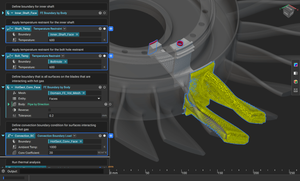
5. Define Boundary Conditions and Run Thermal Analysis
Use the Temperature Restraint block to define the temperature at the shaft and bolt hole, then use a Convection Boundary Load block to capture the heat transfer on the blades and outer shaft face from the hot flow.
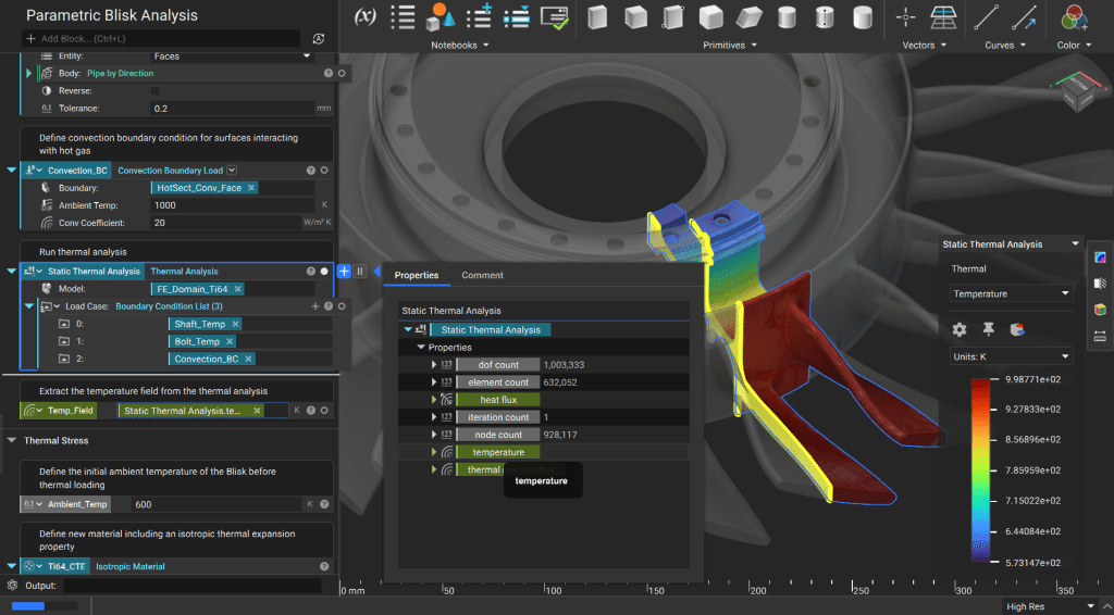
Run a Thermal Analysis using the defined boundary conditions and pull out the temperature field result from the properties tab so we can use it to define thermal stress.
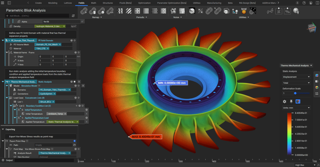
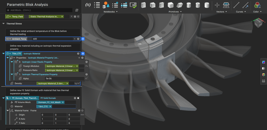
6. Set Up and Run Thermo Mechanical Analysis
Start by defining an ambient temperature before the thermal load is applied, then define a new material that includes a Thermal Expansion Property (we use an isotropic material, but it can be orthotropic or anisotropic) and create a new FE Solid Domain.
Finally, re-run a static analysis using the newly defined FE Domain, adding Initial Temperature and Applied Temperature Load boundary conditions to the initially defined mechanical boundary conditions. Use the temperature field result as the input to the “Applied Temperature Load” boundary condition.
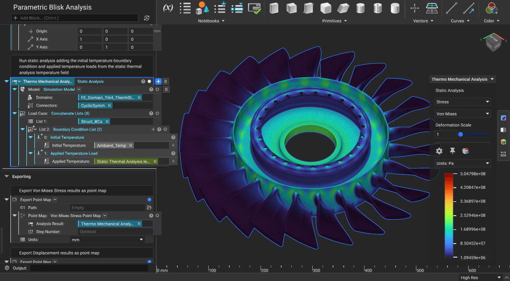
You can then export the displacement or stress/strain results of your Thermo-Mechanical analysis as a point map for further analysis. You can also use maximum values as inputs to objectives or constraints in the formulation of a design optimization problem.