Modeling Aircraft Ducts
Let’s now establish a workflow that generates our ducting geometry. In this example, our output will be an implicit field that defines the duct’s interior volume, a representation we can use to offset into solid duct walls or subtract from our fuselage to carve out the airflow passages.
Following the approach from our Modeling a Single Panel Wing lesson, we’ll create a unilateral duct first, then apply the Mirror Body Symmetrically custom block to generate matching ducts on both sides of the fuselage.
This workflow will demonstrate how parametric design allows you to quickly explore different duct configurations by simply adjusting the input parameters, while maintaining all the complex geometric relationships that ensure intended airflow transitions.
We will accomplish this through the following major steps:
- Set a planar path to define the duct centerline and flow direction.
- Generate a ramped profile to control the cross-sectional shape transition.
- Make a planar duct along the profile using field-based operations.
- Remap duct in the z direction to implement 3D spatial positioning.
Feel free to use the starter file containing only the initial inputs to follow along.
Downloadable Files:
This file was last updated in nTop 5.30.2
1. Planar Profile
Set a planar path to define the duct centerline and flow direction.
Ultimately, our ducting will exist in all 3 dimensions of our coordinate system. Let’s simplify this, beginning with only the x and y coordinates, and saving z for later. In this step, we will establish the path in the xy plane that one side of our ducting will follow. Again, we will begin by modeling the ducting unilaterally, then mirroring later on for simplicity.
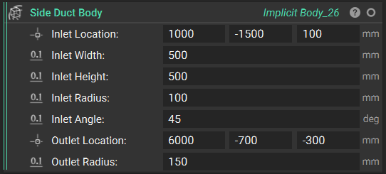
Some additional parameters we’ll use to control the path are
- Butt Line Zero to establish the aircraft’s centerline symmetry plane.
- Path Start/End Tension to control how “stiff” the spline curve is at its endpoints
- Transition Continuity to set the mathematical smoothness level for all transitions in the workflow
For the spline geometry, we’ll extract the x and y coordinates from our inlet and outlet locations, but deliberately force the z-coordinate to zero. This flattens our 3D routing problem into a manageable 2D “top view” path that we can easily control and visualize.

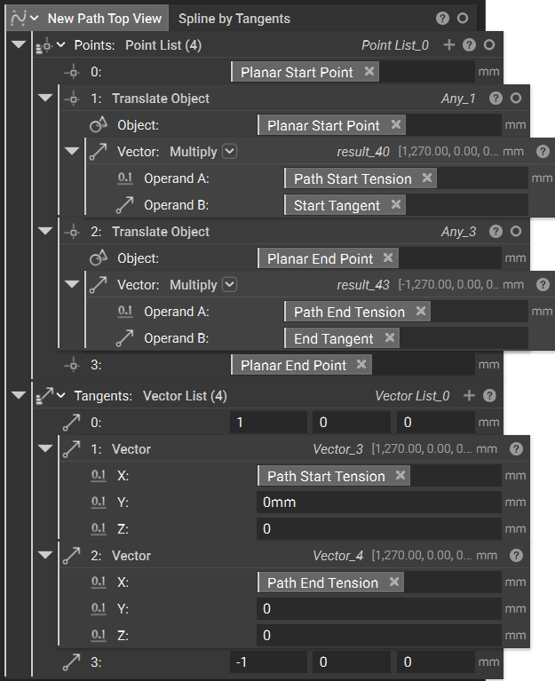
For directional control, we assign start and end tangent vectors pointing in opposite x-directions, positive at the inlet, and negative at the outlet. These opposing tangents naturally create an S-curve that flows smoothly from inlet to outlet along the aircraft’s longitudinal axis.

For the spline construction, we use a four-point system where the middle control points are calculated by translating each endpoint along its respective tangent vector, scaled by the tension value. This gives us precise control over entry and exit curvature while allowing natural flow in between.
Finally, we convert this 2D spline into a profile object with a z-direction extrusion vector, preparing it for the 3D operations that will follow in subsequent steps.
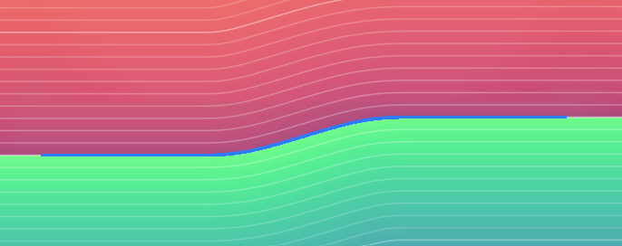
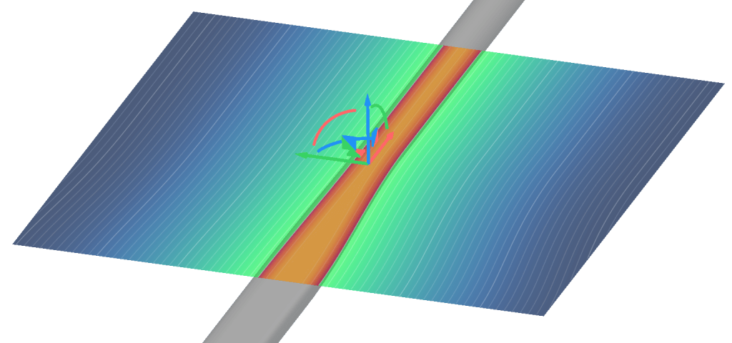
From the resulting spline, we see a fully positive SDF radiating from the spline.

We generate a profile from the top view using Profile from Curves to generate an implicit SDF, where one side of the open curve is positive and the other is negative. We’ll use this resulting field later on when we generate and mirror the duct.
Feel free to follow along and create the planar profile using the video below.
2. Ramped Profile
Generate a ramped profile to control the cross-sectional shape transition.
Now, let’s generate a ramped parallelogram profile like the one that will form our duct cross-section. We’ll use a custom block to help simplify our overall workflow.
Our goal in this step is to create a parametric shape that transitions smoothly from the inlet’s rectangular geometry to the outlet’s circular geometry along our spline path.
You can take different approaches when creating your duct cross-section:
- Simple geometric approach: Use basic rectangles or circles that change size along the path
- Parametric parallelogram approach: Create angled, blended shapes that optimize airflow characteristics
- Custom profile approach: Import or manually define complex cross-sectional shapes
This custom block uses the parametric parallelogram approach because it provides the aerodynamic benefits of angled sides while maintaining smooth geometric transitions.
At the inlet, we generate the cross-sections of the duct, assigning parallelogram cross-section. For the outlet, we assign a circular cross-section. We define these geometries with the parameters shown below.

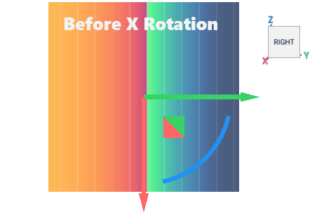
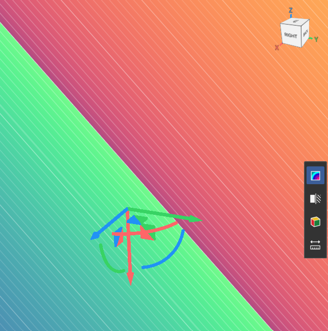
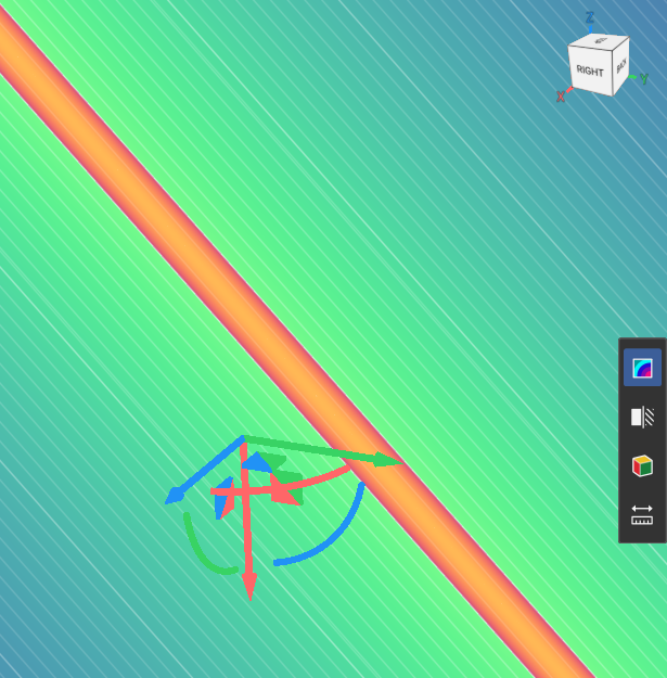
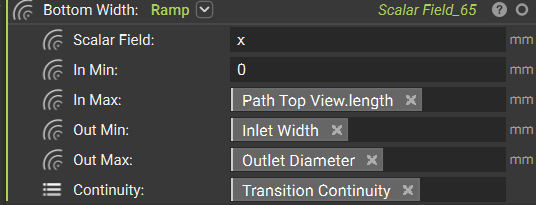
For the basic width setup, the workflow takes the bottom width input and divides it by two to create a “Half Width” value. This establishes the symmetric foundation needed for the parallelogram construction. To adjust our coordinate system for the angled geometry, we use the custom block X Rotation to modify the scalar field y (interchangeable with the xz plane). We perform a 3D rotation around the X-axis by applying trigonometric transformations to remap Y and Z coordinates while preserving the X coordinate.
Downloadable Files:
This file was last updated in nTop 5.30.2
We then displace the resulting scalar field by shifting its coordinate system a Half Width in the y-direction to align it with our intended inlet.

We displace the negative of this result by the negative of the bottom width to create a displaced and opposite field.
We intersect the two resulting fields to generate the angled sides of the parallelogram.
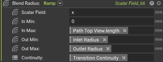
We then intersect this field with the z field (offset by the height) and the -z field to create the horizontal boundaries of the parallelogram. In this step, we can also pull in the Blend Radius. The result is a single implicit field representing the complete parallelogram cross-section.

You can download the resulting custom block below to use in your own workflow.
Downloadable Files:
This file was last updated in nTop 5.30.2
Now we can implement the gradual change from a parallelogram to a circular cross section as we move from the inlet location to the outlet location.
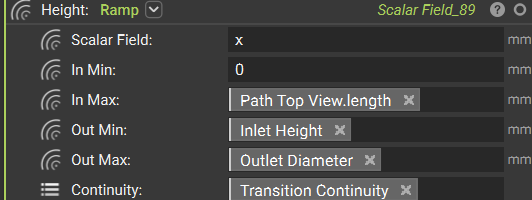
To do this, we will use Ramps instead of scalars as inputs in the CB above. Each ramp will output a scalar field that varies from along the length field of Path Top View, so we will see a transition from the inlet location, zero, to the outlet location, Total Path Length.
We can assign our pre-defined transition continuity to each of these ramps.

The output of this is an infinite duct that ramps from a parallelogram at its inlet to a circle at its outlet.
Feel free to walk through the custom block and underlying fields in the video below.
3. Planar Duct
Make a planar duct along the profile using field-based operations.
Now let’s modify the geometry we created above to:
- Follow our planar path
- Mirror the result to generate bilateral ducts
- Align with our inlet location (we’ll handle outlet alignment in the final step to compensate for any z-coordinate mismatches)
To make the ramped parallelogram follow the planar path, we’ll use a Remap Field block to reassign the coordinates:
- x: Spline length field
- y: Distance to extrusion (the SDF representing distance from any point to the infinite extrusion of the profile)
- z: Negative z-coordinate
After remapping, we apply the Mirror Body Symmetrically custom block (used earlier in the course) to mirror the duct across the butt line, creating the bilateral duct configuration.
Downloadable Files:
Mirror Body Symmetrically.ntop
This file was last updated in nTop 5.30.2
Finally, we translate the resulting field in the z-direction by the inlet z-coordinate plus half of the inlet height. This positions the entire planar duct system at the correct inlet elevation.
See the video below to follow along.
4. 3D Duct
Remap duct in the z direction to implement 3D spatial positioning.
In these final steps, we’ll apply displacement fields in the z-direction to compensate for elevation differences between the inlet and outlet locations.
To handle this vertical offset, we’ll use the Displace block.
We can set the x and y displacements to zero, since we’ve already accounted for the top-view duct profile in our earlier sketching.
To achieve a smooth z-direction transition we will:
- Use the Two Body Field between planes positioned at the inlet and outlet locations
- Feed this field into a Ramp function
- Apply linear z-displacement from inlet to outlet elevation (this can be adjusted for non-linear displacement if preferred)

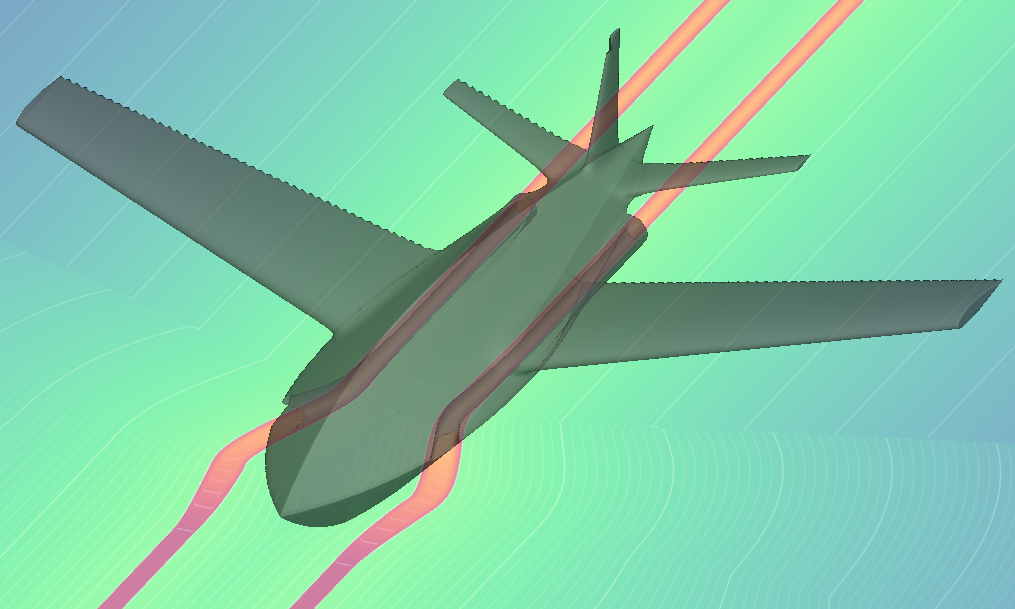
At this point, we have an infinite, bilateral duct that properly accounts for changes in all three directions (x, y, and z). We’ll add bounds to limit the duct geometry to the specific region between inlet and outlet, preventing the infinite field from extending beyond the intended duct length.

Feel free to take a look at this process in the video below.