Topology Optimization Properties and Terminology

TopOpt is an iterative process that updates the topology until the objective is reached and the constraints are satisfied. If the process is taking a long time, the user can set a maximum limit to the number of iterations attempted. This input allows you to limit the maximum computation time expended on the TopOpt process. 

The objective function is a quantified measure of how well the topology is achieving its objective(s). When the relative change between iterations of the objective function falls below this number, the TopOpt will be considered complete (as long as the constraints are satisfied). Decreasing this number will result in a more accurate TopOpt, but longer computation time.

This input is a convergence threshold, like described above, but for the relative change of the elements TopOpt density from one iteration to the next. Decreasing this number will result in a more accurate TopOpt, but longer computation time.

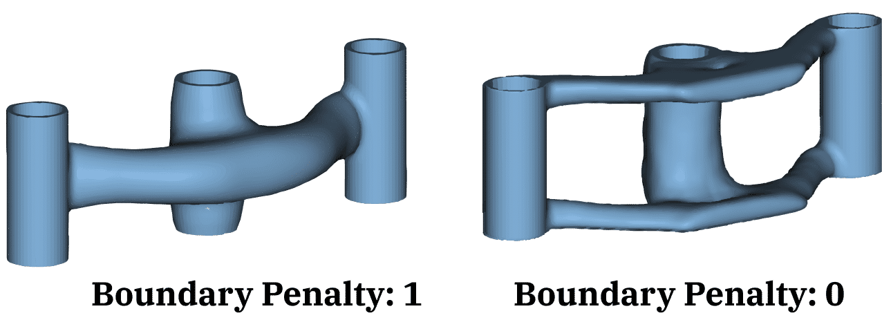
This input controls how the TopOpt deals with setting density values at the edges of the design space. An input of 1 sets the TopOpt density to 0 along the edges of the design space. The material will be completely restricted on the boundary where no loads or constraints have been applied. This option works well if you set up your design space to have a buffer zone of nodes on the outside of the space where you know that no material will be filled in. In some cases, you may anticipate that your part will end up including elements on the outer edge of the design space. This is likely true if you are doing TopOpt on a coarse mesh. An input of 0 defines TopOpt densities at the design space edges such that the gradient (the spatial derivatives in x,y,z) will be zero. This allows you to have non-zero TopOpt densities at edges. No penalization is enforced on the boundary in this case. The overall recommendation is to use a small enough mesh size so that the 1 option can be used and density can be 0 at the edges, but if needed, option 0 provides an alternative. The image below shows how results can change between different Filter Boundary options.

This input controls the amount of data stored and accessible after the topology optimization completes. The number can be increased to lower the file size of a completed TopOpt file. The default value of 1 will save results for all increments, whereas a result of 0 will save only the first and last increment. For any value, N, greater than 1, it will save results for every N increments. Note: The last iteration will always be saved.

This optional input specifies a minimum feature size that will be present in your TopOpt result. Note that it can accept a field input, meaning you can choose a spatially-variant scalar field as your minimum feature size. If this optional input is left blank, we assume a default value of 2 times the average element size.

This optional input can take in a scalar field of TopOpt density values (from 0 to 1), which will provide the initial guess at the TopOpt result before the process begins. When left blank, the TopOpt densities are set to 0.5 at all elements.